以下是实现对图形对象的相对比例的精确控制所需的步骤。
要实现一致的比例,需要显式指定输入坐标范围(常规坐标)和输出坐标范围(绝对坐标)。规则坐标范围取决于
PlotRange
,
PlotRangePadding
(可能还有其他选择?).绝对坐标范围取决于
ImageSize
,
ImagePadding
(可能还有其他选择?)。对于
GraphPlot
,仅需指定
绘图范围
和
图像大小
.
要创建按预定比例呈现的图形对象,您需要了解
绘图范围
需要完全包含对象,对应
图像大小
然后回来
Graphics
指定了这些设置的对象。找出必要的
绘图范围
当涉及到粗线条时,处理起来更容易
AbsoluteThickness
,称之为
abs
. 要完全包含这些行,您可以采取最小的
绘图范围
它包括端点,然后通过ABS/2偏移最小X和最大Y边界,并通过(ABS/ 2+1)偏移最大X和最小Y边界。注意这些是输出坐标。
当组合几个
scale-calibrated
需要重新计算的图形对象
PlotRange/ImageSize
并为组合图形对象显式设置它们。
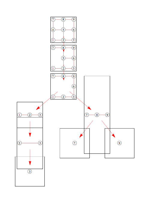
插入
刻度盘校准
对象到
葡萄园
你需要确保自动
葡萄园
定位在同一范围内。为此,您可以选择几个角节点,手动确定它们的位置,然后让自动定位来完成其余的工作。
原语
Line
/
JoinedCurve
/
FilledCurve
根据直线是否(几乎)共线,以不同的方式渲染连接/封口,因此需要手动检测共线性。
使用这种方法,渲染图像的宽度应该等于
(inputPlotRange*scale + 1) + lineThickness*scale + 1
第一个额外的
1
是为了避免“fencepost错误”,第二个额外的1是需要添加在右边的额外像素,以确保粗线不被截断
我已经验证了这个公式
Rasterize
论合并
Show
并使用
Texture
并以
Orthographic
投影结果与预测结果吻合。对对象执行“复制/粘贴”
Inset
进入之内
葡萄园
,然后光栅化,得到的图像比预期的薄一个像素。

(来源:
yaroslavvb.com
)
(**** Note, this uses JoinedCurve and Texture which are Mathematica 8 primitives.
In Mathematica 7, JoinedCurve is not needed and can be removed *)
(** Global variables **)
scale = 50;
lineThickness = 1/2; (* line thickness in regular coordinates *)
(** Global utilities **)
(* test if 3 points are collinear, needed to work around difference \
in how colinear Line endpoints are rendered *)
collinear[points_] :=
Length[points] == 3 && (Det[Transpose[points]~Append~{1, 1, 1}] == 0)
(* tales list of point coordinates, returns plotRange bounding box, \
uses global "scale" and "lineThickness" to get bounding box *)
getPlotRange[lst_] := (
{xs, ys} = Transpose[lst];
(* two extra 1/
scale offsets needed for exact match *)
{{Min[xs] -
lineThickness/2,
Max[xs] + lineThickness/2 + 1/scale}, {Min[ys] -
lineThickness/2 - 1/scale, Max[ys] + lineThickness/2}}
);
(* Gets image size for given plot range *)
getImageSize[{{xmin_, xmax_}, {ymin_, ymax_}}] := (
imsize = scale*{xmax - xmin, ymax - ymin} + {1, 1}
);
(* converts plot range to vertices of rectangle *)
pr2verts[{{xmin_, xmax_}, {ymin_, ymax_}}] := {{xmin, ymin}, {xmax,
ymin}, {xmax, ymax}, {xmin, ymax}};
(* lifts two dimensional coordinates into 3d *)
lift[h_, coords_] := Append[#, h] & /@ coords
(* convert Raster object to array specification of texture *)
raster2texture[raster_] := Reverse[raster[[1, 1]]/255]
Subset[a_, b_] := (a \[Intersection] b == a);
inducedGraph[set_] := Select[edges, # \[Subset] set &];
values[dict_] := Map[#[[-1]] &, DownValues[dict]];
(** Graph Specific Stuff *)
graphName = {"Grid", {3, 3}};
verts = Range[GraphData[graphName, "VertexCount"]];
edges = GraphData[graphName, "EdgeIndices"];
vcoords = Thread[verts -> GraphData[graphName, "VertexCoordinates"]];
jedges = {{{1, 2, 4}, {2, 4, 5, 6}}, {{2, 3, 6}, {2, 4, 5, 6}}, {{4,
5, 6}, {2, 4, 5, 6}}, {{4, 5, 6}, {4, 5, 6, 8}}, {{4, 7, 8}, {4,
5, 6, 8}}, {{6, 8, 9}, {4, 5, 6, 8}}};
jnodes = Union[Flatten[jedges, 1]];
(* Generate diagram with explicit PlotRange,ImageSize and \
AbsoluteThickness *)
plotHL[verts_, color_] := (
coords = verts /. vcoords;
obj = JoinedCurve[Line[coords],
CurveClosed -> Not[collinear[coords]]];
(* Figure out PlotRange and ImageSize needed to respect scale *)
pr = getPlotRange[verts /. vcoords];
{{xmin, xmax}, {ymin, ymax}} = pr;
imsize = scale*{xmax - xmin, ymax - ymin};
lineForm = {Opacity[.3], color, JoinForm["Round"],
CapForm["Round"], AbsoluteThickness[scale*lineThickness]};
g = Graphics[{Directive[lineForm], obj}];
gg = GraphPlot[Rule @@@ inducedGraph[verts],
VertexCoordinateRules -> vcoords];
Show[g, gg, PlotRange -> pr, ImageSize -> imsize]
);
(* Initialize all graph plot images *)
SeedRandom[1]; colors =
RandomChoice[ColorData["WebSafe", "ColorList"], Length[jnodes]];
Clear[bags];
MapThread[(bags[#1] = plotHL[#1, #2]) &, {jnodes, colors}];
(** Ploting parent graph of subgraphs **)
(* figure out coordinates of subgraphs close to edges of bounding \
box, use them to anchor parent GraphPlot *)
bagCentroid[bag_] := Mean[bag /. vcoords];
findExtremeBag[vec_] := (vertList = First /@ vcoords;
coordList = Last /@ vcoords;
extremePos =
First[Ordering[jnodes, 1,
bagCentroid[#1].vec > bagCentroid[#2].vec &]];
jnodes[[extremePos]]);
extremeDirs = {{1, 1}, {1, -1}, {-1, 1}, {-1, -1}};
extremeBags = findExtremeBag /@ extremeDirs;
extremePoses = bagCentroid /@ extremeBags;
(* figure out new plot range needed to contain all objects *)
fullPR = getPlotRange[verts /. vcoords];
fullIS = getImageSize[fullPR];
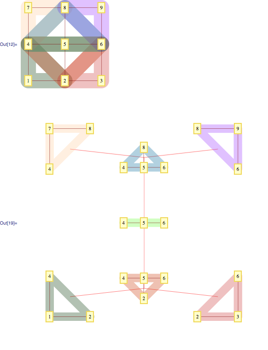
(*** Show bags together merged ***)
image1 =
Show[values[bags], PlotRange -> fullPR, ImageSize -> fullIS]
(*** Show bags as vertices of another GraphPlot ***)
GraphPlot[
Rule @@@ jedges,
EdgeRenderingFunction -> ({Gray, Thick, Arrowheads[.05],
Arrow[#1, 0.22]} &),
VertexCoordinateRules ->
Thread[Thread[extremeBags -> extremePoses]],
VertexRenderingFunction -> (Inset[bags[#2], #] &),
PlotRange -> fullPR,
ImageSize -> 3*fullIS
]
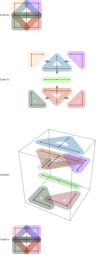
(*** Show bags as 3d slides ***)
makeSlide[graphics_, pr_, h_] := (
Graphics3D[{
Texture[raster2texture[Rasterize[graphics, Background -> None]]],
EdgeForm[None],
Polygon[lift[h, pr2verts[pr]],
VertexTextureCoordinates -> pr2verts[{{0, 1}, {0, 1}}]]
}]
)
yoffset = 1/2;
slides = MapIndexed[
makeSlide[bags[#], getPlotRange[# /. vcoords],
yoffset*First[#2]] &, jnodes];
Show[slides, ImageSize -> 3*fullIS]
(*** Show 3d slides in orthographic projection ***)
image2 =
Show[slides, ViewPoint -> {0, 0, Infinity}, ImageSize -> fullIS,
Boxed -> False]
(*** Check that 3d and 2d images rasterize to identical resolution ***)
Dimensions[Rasterize[image1][[1, 1]]] ==
Dimensions[Rasterize[image2][[1, 1]]]


